가전제품 이것저것 이야기

논문 링크

https://arxiv.org/pdf/1311.2524.pdf

2014년 발행

0. TITLE

Rich feature hierarchies for accurate object detection and semantic segmentation

: 정확한 detection과 segmentation을 위한 feature 계층화

1. Abstract

최근 Object Detection 성능이 정체되었다.

PASCAL VOC dataset에서 가장 높은 수준을 달성한 방식은 다수의 low-level image feature 들을 high-level context와 결합한 것이었다.

이 논문에서는 이전 최고 모델(VOC 2012에서 mAP 53.3%) 보다 mAP 기준 30% 향상시킨 알고리즘을 소개하려고 한다.

우리 알고리즘의 핵심 요소는 

1) bottom-up region proposals에 높은 용량의 CNN을 적용할 수 있다는 것 (localize와 segment를 위해)

2) labeled 학습 데이터가 부족할 때, 보조 작업에 대한 supervised pre-training(domain-specific한 fine-tuning)이 엄청난 성능 향상을 가져다줌

-> (image classification) 의 충분한 데이터로 보조 작업을 하고 target task(detection)으로 fine-tune하는 방식

우리는 CNN과 함께 region proposals들을 결합하였기 때문에

우리의 알고리즘을 R-CNN(Regions with CNN features)라고 부르기로 하였다.

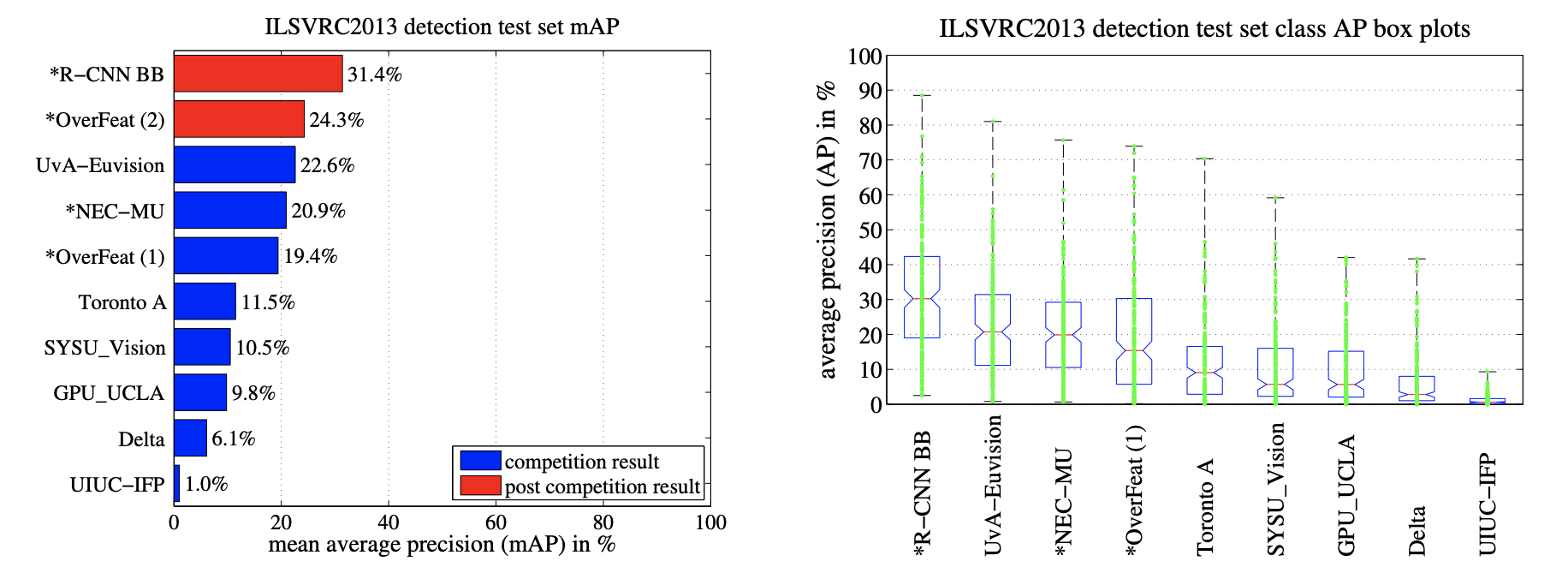
우리는 OverFeat라는 비슷한 CNN 구조를 가진 sliding window detector를 제안한 모델과 R-CNN을 비교하였다.

200-class ILSVRC2013 detection dataset에서 R-CNN이 OverFeat의 성능을 능가했다는 것을 증명하였다

2. Conclusion 

우리 알고리즘의 두가지 인사이트

1) bottom-up region proposals에 높은 용량의 CNN을 적용할 수 있다는 것 (localize와 segment를 위해)

2) 데이터가 부족한 문제에 “supervised pre-training/domain-specific finetuning"이 굉장히 효과적이다.

3. Result & Discussion (Data 훑기)

1) Object detection with R-CNN

- Results on PASCAL VOC 2010-12

bounding box regression이 있는 것과 없는 결과로 두가지 제출하였다.

non-linear kernel SVM approach로 mAP 기준 35.1% -> 53.7%로 향상 + 더 빠름

- Results on ILSVRC2013 detection

PASCAL VOC에서 사용한 하이퍼 파라미터와 동일하게 설정

bounding box regression이 있는 것과 없는 결과로 두가지 제출하였다.

2) Semantic segmentation

- Results on VOC 2011

[ validation results ]

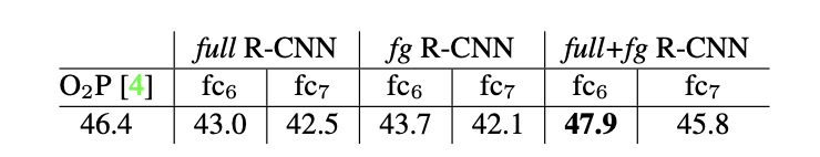
fg strategy가 full strategy보다 약간 더 성능이 좋다.

이는 masked region shape가 더 강력한 signal을 보낸다는 것이다.

full+fg의 성능이 더 좋다.

즉, full features에 의해 제공받은 context가 유익하다는 것이다. 

게다가 10시간 이상 걸렸던 O2P와  다르게, 20 SVR에 우리의 full-fg features를 적용한 것은 1시간에 안에 학습이 완료되었다. 

[ test results ] 

21개의 카테고리 중에 우리의 모델(full+fg R-CN fc6)이 11개의 카테고리에서 가장 높은 성능을 기록했다.

또한, overall 로서는 47.9로 가장 높은 수치를 기록하였다.

4. Introduction

이 논문은 CNN이 PASCAL VOC의 object detection task에서도 놀라운 성능을 보여줄 수 있다는 것을 첫번째로 보여줄 것이다.

두 가지에 집중하였다.

1) 깊은 신경망에서 localizing하는 것

2) 적은 object detection 데이터로도 높은 용량의 모델을 학습시키는 것

classification과는 다르게, object detection은 localizing object하는 것이 필요하다.

하지만, CNN은 굉장히 큰 receptive fields와 stride를 가지고 있기 때문에 sliding-window 방식을 적용하기에 어려움이 있다.

우리는 이를 "recognition using regions" 파라다임을 적용함으로써 해결하였다. -> object detection과 semantic segmentation에 모두 성공적이었다.

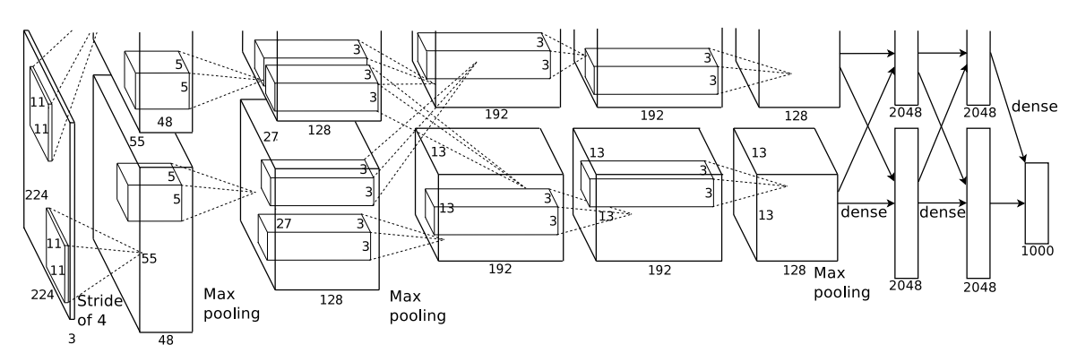
1) input image를 넣는다

2) 약 2000개의 bottom-up region proposals들을 추출한다 -> affine image warping을 적용하여 input size 통일

3) 각각의 proposal에 큰 CNN를 적용하여 고정 크기의 feature vector를 추출한다.

4) 각각의 region을 class-specific linear SVM을 적용하여 분류한다

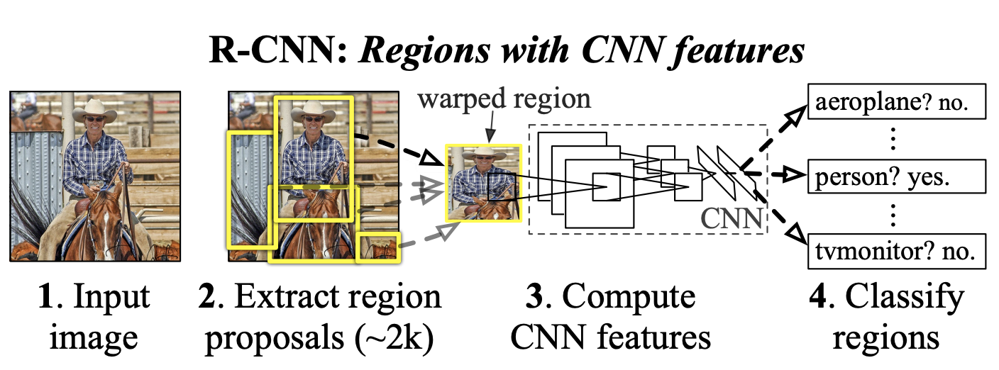
* affine image warping 기법을 이용하여, 각각의 region proposal로부터 고정 크기의 input image를 얻음

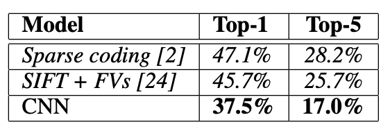
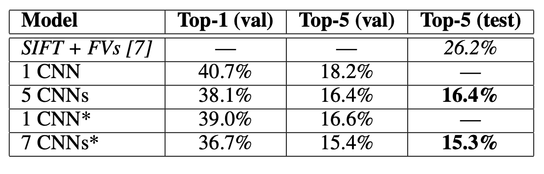
-> sliding-window 방식을 사용한 OverFeat model보다 성능이 높다. (mAP 기준)

두 번째 문제는, 큰 CNN을 적용하기에 레이블된 데이터가 부족하다는 것이었다.

기존의 전통적인 해결방식은 unsupervised pre-training과 supervised fine-tuning을 사용하는 것이었는데,

우리는 1) 대규모의 보조 데이터셋에(ILSVRC) supervised pre-training을 적용하고

2) 작은 데이터셋(PASCAL)에 domain-specific한 fine-tuning을 적용하는 방식을 이용하였다.

이는, 데이터가 적을 때 높은 용량의 CNN을 학습시키는 데에 효과적이었다.

우리의 실험에서 detection을 위한 fine-tuning을 통해 mAP를 8%point나 올릴 수 있었다. 

논문 링크

https://proceedings.neurips.cc/paper/2012/file/c399862d3b9d6b76c8436e924a68c45b-Paper.pdf

2012년 발행

0. TITLE

ImageNet Classification with Deep Convolutional Neural Networks

: CNN을 이용해서 ImageNet 데이터에 classification task를 수행한다.

1. Abstract

ImageNet LSVRC-2010 contest에 나왔던 1.2 백만개의 데이터를 1000개의 클래스로 분류하는 작업이다.

top-1과 top-5 error rate가 각각 37.5%, 17%로 이전 SOTA 모델보다 개선된 수치를 달성하였다.

[ 구조 ]

6천만개의 파라미터와 65만개의 뉴런을 가진 뉴럴 네트워크가

5개의 convolution layers로 이루어져 있다.

이 중 일부는 max-pooling layer와 3개의 fully connected layer로 이어진다.

마지막은 1000개로 softmax.

[ 성능 향상을 위해 ]

fully connected layer의 overfitting을 줄이기 위해

"dropout"이라는 정규화 기법 사용

2. Results & discussion (data 훑기)

1) ILSVRC2010 test set 에 대한 error rates 비교

2) ILSVRC-2012 validation과 test sets에 대한 error rates 비교

(asterisk*가 붙은 것은 ImageNet 2011 Fall release 데이터로 “pre-trained”한 것)

3) Discussion

한 개라도 convolution layer가 사라진다면, 성능이 크게 저하된다. 

top-1  performance에서도 중간에 한 layer를 삭제했더니 2%의 성능 감소가 있었다.

따라서, depth는 결과에 있어 아주 중요한 요소이다.

학습에 있어서 unsupervised pre-training을 사용하지 않았다.

궁극적으로는 video sequences에 크고 깊은 convolution nets를 사용하여 

도움이 되는 정보를 제공하는 것이 목표이다.

3. Introduction

간단한 recognition task는 작은 데이터셋으로도 풀 수 있었지만,

실제 물체는 상당한 다양성을 가지고 있기 때문에 더 큰 training set를 사용해야만 한다.

수만은 물체들을 인식하기 위해서는 더 큰 용량을 가진 모델이 필요해졌다.

게다가 주어지지 않은 이미지들에 대한 고려도 해야한다.

이러이러한 문제점이 있지만,

다행히도 현재의 강력한 GPU와 오버피팅없이 train할 수 있을만큼 많은 레이블된 데이터가 있어

문제를 해결할 수 있다.

우리의 모델은 가장 큰 CNN 모델 중의 하나를 학습시켰고,

ILSVRC-2010 and ILSVRC-2012에서 가장 높은 결과를 얻을 수 있었다.

두 개의 GTX 580 3GB GPU로 5-6일간 학습시켰다.

우리의 실험은 더 빠른 GPU와 더 큰 데이터셋이 있다면 결과가 더 개선될 수 있음을 제안하였다.

4. Architecture

5개의 convolution layer + 3개의 fully-connected layer

1) ReLU의 Non-linearity

기존의 sigmoid나 tanh는 ReLU보다 훨씬 느리다. 즉, ReLU가 훨씬 빠르다.

ReLU는 기존의 activation 함수들보다 경사 하강 알고리즘에 유리하며, overfitting 감소하는 장점이 있다.

ReLU(solid), tanh(dashed) 비교 그래프

f(x) = |tanh| 함수로도 시도가 있었지만, 여기서는 overfitting을 막는 데에 초점이 맞춰져 있었기 때문에

우리가 발표한 ReLU를 사용할 때 발생되는 accelerated ability와는 다르다 

2) 2개의 GPU 사용

1.2백만개의 training 데이터를 사용하기에 1개의 GPU로는 충분치 않아서

두 개의 GPU 사용하였다. 

parallelization 기법 사용하였다.

kernel을 반으로 나눠 각각의 GPU에 넣고, 특정 layer에서 communication 하는 방식

3) Local Response Normalization 국지 정규화

정규화가 일반화에 영향을 준다는 것을 알아냈다.

k = 2, n = 5, α = 10−4, β = 0.75 는 여러 연구를 통해 알아낸 최적의 수치이며 

이는 하이퍼 파라미터이다. 아래의 식에 적용하여 정규화(normalization) 수행

* 해당 Normalization 방식을 ReLU 뒤에 수행하였다. 성능향상에 효과적이었다.

4) Overlapping pooling

pooling layer에서 s(stride) < z(filter size) 하게 만들어서

overlap 하게 만들었다. 성능향상에 효과적이었다.

5) 전체 구조

[ 모델 구조 ]

두 번째, 네 번째, 다섯 번째 convolution layer는 동일한 GPU에 있었던 이전 layer와만 연결되어 있다.

세 번째 Layer은 두 번째 layer의 모든 kernel map과 연결되어 있다.

fully-connect layer들은 모든 이전의 kernel map과 연결되어 있다.

첫번째, 두번째 convolution layer에서 LRN을 사용하였다.

max-pooling은 LRN 뒤에랑 다섯번째 convolution layer에서 사용하였다.

ReLU non-linearity는 모든 convolution layer와 fully-connected layer에서 사용되었다.

[ 필터 크기 ]

첫번째 convolution layer의 필터는 224x224x3 input images + 96개의 11x11x3 kernel + 4 pixel의 stride

두번째 convolution layer의 필터는 첫번째 layer의 output size(LRN과 max-pooling 적용된) + 256 kernels of size 5 × 5 × 48 The third, fourth, and fifth convolutional layers are connected to one another without any intervening pooling or normalization layers.

The third convolutional layer has 384 kernels of size 3 × 3 × 256 connected to the (normalized, pooled) outputs of the second convolutional layer.

The fourth convolutional layer has 384 kernels of size 3 × 3 × 192 , and

the fifth convolutional layer has 256 kernels of size 3 × 3 × 192. The fully-connected layers have 4096 neurons each.

5. Overfitting을 줄이기 위해

1) Data Augmentation

label-preservatin transformations를 사용하여 데이터셋을 인위적으로 늘리는 방식 사용하였다.

data augmentation은 CPU에서 실행하였으므로 computationally free하다.

- The first form of data augmentation

generating image translations & horizontal reflections

(random 224 × 224 patches)

-> softmax

- The second form of data augmentation

altering the intensities of the RGB channels in training images

Specifically, PCA on the set of RGB pixel values

add multiples of the found principal components with magnitudes proportional to the corresponding eigenvalues times a random variable drawn from a Gaussian with mean zero and standard deviation 0.1.

2) Dropout

여러 다른 모델들의 예측 결과를 합치는 것도 error 줄이는 데에 매우 효과적이다.

하지만, 굉장히 큰 neural network에 쓰기에는 너무 비싸다.

대신에 dropout을 사용하면 매우 효과적이다. (setting to zero the output of each hidden neuron with probability 0.5)

뉴런들끼리의 영향력을 줄여준다.

마지막에 0.5를 곱해준다.

우리는 dropout을 첫 두개의 fully-connected layer에 적용하였다.

6. Details of learning

stochastic gradient descent를 사용하였다.

batch size 128

momentum 0.9

weight decay 0.0005(중요함) -> 정규화 뿐만 아니라 training error를 줄여줬음

모든 layer에 동일한 Learning Rate 적용하였음 -> lr = 0.01

epoch = 90